Get help with Advanced Functions, Grade 12 (University)
Most tutoring makes you sit through material you already know. MapleMind flips that: pick the exact skill that's causing trouble — any of the 72 below — and the tutor teaches just that one, step by step, as many times as it takes. Ask questions in plain words, any time of day, in English, French, or 12 other languages.
The official Ontario Advanced Functions, Grade 12 (University) curriculum
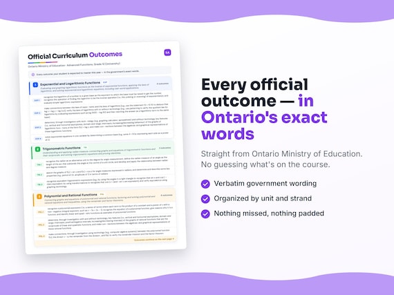
Ontario defines Advanced Functions, Grade 12 (University) by strands and outcomes. MapleMind teaches the same curriculum reorganized for one-skill-at-a-time tutoring — the table shows exactly where every official strand lands, and the ministry's own wording is quoted under each unit below.
Official source Ontario's official mathematics curriculumRead it on the government site — dcp.edu.gov.on.ca ↗| Official strand | Outcomes | Where MapleMind teaches it |
|---|---|---|
| Strand 1 | 14 | Exponential and Logarithmic Functions |
| Strand 2 | 16 | Trigonometric Functions |
| Strand 3 | 22 | Polynomial and Rational Functions |
| Strand 4 | 20 | Characteristics of Functions |
Every skill below, taught one on one.
 Try the first session free
How MapleMind teaches Advanced Functions, Grade 12 (University) — every unit, lesson, and skill
Every skill below runs as a short session: a plain-words lesson, a worked example, solving it together, then a five-question skill check that earns up to three stars. Guided Mode keeps it teaching instead of answer-handing — turning it off needs a parent's password.
Unit 1Exponential and Logarithmic FunctionsOfficial strand · Strand 1
Evaluating and graphing logarithmic functions as the inverse of exponential functions, applying the laws of logarithms, and solving exponential and logarithmic equations, including real-world applications.
Evaluating Logarithmic Expressions
- The logarithm as the inverse of exponentiationmhf4u.1.1 — Recognize the logarithm of a number to a given base as the exponent needed to raise the base to get the number, recognize that finding a logarithm undoes exponentiation, and evaluate simple logarithmic expressions.
- Approximating logarithms with technologymhf4u.1.2 — Determine, with technology, the approximate logarithm of a number to any base, including base 10, by systematic trial.
- Connecting logarithmic and exponential equationsmhf4u.1.3 — Make connections between a logarithmic equation and its equivalent exponential equation.
The Laws of Logarithms
- Deriving and verifying the laws of logarithmsmhf4u.1.4.a — Make connections between the laws of exponents and the laws of logarithms, and verify the laws of logarithms with or without technology.
- Applying the laws of logarithms to simplify and evaluatemhf4u.1.4.b — Use the laws of logarithms to simplify and evaluate numerical expressions.
Connecting Graphs and Equations of Logarithmic Functions
- Key features of the graph of f(x) = log xmhf4u.1.5 — Determine, through investigation with and without technology, the key features (asymptotes, domain and range, intercepts, increasing/decreasing behaviour) of the graphs of logarithmic functions, and connect the algebraic and graphical representations.
- Logarithmic and exponential functions as inversesmhf4u.1.6 — Recognize that an exponential function and its corresponding logarithmic function are inverses, deduce that their graphs reflect in the line y = x, and verify with technology.
- The roles of parameters in transformed logarithmic functionsmhf4u.1.7 — Determine, through investigation using technology, the roles of the parameters d, c, a, and k in transformed logarithmic functions, and describe these roles as transformations.
- Solving real-world exponential and logarithmic problems from a graphmhf4u.1.8 — Pose problems based on real-world applications of exponential and logarithmic functions, and solve them using a given graph or a graph generated with technology.
- Simplifying equivalent logarithmic and exponential expressionsmhf4u.1.9 — Recognize equivalent algebraic expressions involving logarithms and exponents, and simplify expressions of these types.
Solving Exponential and Logarithmic Equations
- Solving exponential equations by finding a common basemhf4u.1.10.a — Solve exponential equations in one variable by expressing both sides as powers of a common base.
- Solving exponential equations using logarithmsmhf4u.1.10.b — Solve exponential equations in one variable by taking the logarithm of both sides, recognizing that base-10 logarithms are commonly used.
- Solving simple logarithmic equations algebraicallymhf4u.1.11 — Solve simple logarithmic equations in one variable algebraically.
- Solving real-world problems with exponential and logarithmic equationsmhf4u.1.12 — Solve problems involving exponential and logarithmic equations algebraically, including problems arising from real-world applications.
The official wording — 14 outcomes in this unit
- mhf4u.1.1
recognize the logarithm of a number to a given base as the exponent to which the base must be raised to get the number, recognize the operation of finding the logarithm to be the inverse operation (i.e., the undoing or reversing) of exponentiation, and evaluate simple logarithmic expressions
- mhf4u.1.2
determine, with technology, the approximate logarithm of a number to any base, including base 10 (e.g., by reasoning that log 29 is between 3 and 4 and using systematic trial to determine that log 29 is approximately 3.07)
- mhf4u.1.3
make connections between related logarithmic and exponential equations (e.g., log 125 = 3
- mhf4u.1.4.a
make connections between the laws of expo- nents and the laws of logarithms [e.g., use the statement 10 = 10 10 to deduce that log x + log y = log (xy)], verify the laws of logarithms with or without technology (e.g., use patterning to verify the quotient law for logarithms by evaluating expressions such as log 1000 – log 100 and then rewriting the answer as a logarithmic term to the same base)
- mhf4u.1.4.b
use the laws of logarithms to simplify and evaluate numerical expressions
- mhf4u.1.5
determine, through investigation with tech- nology (e.g., graphing calculator, spreadsheet) and without technology, key features (i.e., vertical and horizontal asymptotes, domain and range, intercepts, increasing/decreasing behaviour) of the graphs of logarithmic func- tions of the form f(x) = log x, and make con- nections between the algebraic and graphical representations of these logarithmic functions
- mhf4u.1.6
recognize the relationship between an expo- nential function and the corresponding loga- rithmic function to be that of a function and its inverse, deduce that the graph of a loga- rithmic function is the reflection of the graph of the corresponding exponential function in the line y = x, and verify the deduction using technology
- mhf4u.1.7
determine, through investigation using technol- ogy, the roles of the parameters d and c in functions of the form y = log (x – d) + c and the roles of the parameters a and k in func- tions of the form y = alog (kx), and describe these roles in terms of transformations on the horizontal translations; reflections in the axes; vertical and horizontal stretches and compressions to and from the x- and y-axes)
- mhf4u.1.8
pose problems based on real-world applica- tions of exponential and logarithmic functions (e.g., exponential growth and decay, the Richter scale, the pH scale, the decibel scale), and solve these and other such problems by using a given graph or a graph generated with technology from a table of values or from its equation
- mhf4u.1.9
recognize equivalent algebraic expressions involving logarithms and exponents, and simplify expressions of these types
- mhf4u.1.10.a
solve exponential equations in one variable by determining a common base (e.g., solve 4 = 8 by expressing each side as a power of 2)
- mhf4u.1.10.b
and by using logarithms (e.g., solve 4 = 8 by taking the logarithm base 2 of both sides), recognizing that logarithms base 10 are commonly used (e.g., solving 3 = 7 by taking the logarithm base 10 of both sides)
- mhf4u.1.11
solve simple logarithmic equations in one variable algebraically [e.g., log (5x + 6) = 2, log (x + 1) = 1]
- mhf4u.1.12
solve problems involving exponential and logarithmic equations algebraically, includ- ing problems arising from real-world applications
Unit 2Trigonometric FunctionsOfficial strand · Strand 2
Understanding and applying radian measure, connecting graphs and equations of trigonometric functions and their reciprocals, and solving trigonometric equations and proving identities.
Understanding and Applying Radian Measure
- The radian as an alternative angle-measure unitmhf4u.2.1 — Recognize the radian as an alternative unit to the degree, define radian measure as arc length subtending an angle at the centre of a unit circle, and relate radian and degree measure.
- Representing radian measure in terms of π and as a rational numbermhf4u.2.2 — Represent radian measure both in terms of π and as a rational number.
- Trigonometric ratios of angles in radians, with technologymhf4u.2.3 — Determine, with technology, the primary and reciprocal trigonometric ratios of angles expressed in radian measure.
- Exact trigonometric values for special angles in radiansmhf4u.2.4 — Determine, without technology, the exact values of the primary and reciprocal trigonometric ratios for special angles and their multiples up to 2π.
Connecting Graphs and Equations of Trigonometric Functions
- Sketching sine and cosine graphs in radiansmhf4u.2.5 — Sketch the graphs of f(x) = sin x and f(x) = cos x for angles in radians, and determine and describe key properties such as period and amplitude.
- Connecting the tangent ratio to the tangent functionmhf4u.2.6 — Make connections between the tangent ratio and the tangent function using technology, and describe key properties of the tangent function.
- Graphing and describing the reciprocal trigonometric functionsmhf4u.2.7 — Graph the reciprocal trigonometric functions with technology, determine and describe their key properties, and recognize their notations.
- Amplitude, period, and phase shift of sinusoidal functionsmhf4u.2.8 — Determine the amplitude, period, and phase shift of sinusoidal functions given in the form f(x) = a sin(k(x − d)) + c, with angles in radians.
- Sketching transformed sine and cosine graphsmhf4u.2.9 — Sketch graphs of transformed sine and cosine functions by applying transformations, and state the period, amplitude, and phase shift.
- Writing the equation of a sinusoidal function from its graph or propertiesmhf4u.2.10 — Represent a sinusoidal function with an equation, given its graph or its properties, with angles in radians.
- Solving real-world problems with trigonometric functions in radiansmhf4u.2.11 — Pose problems based on applications involving a trigonometric function with a radian domain, and solve them using a given graph or a graph generated with or without technology.
Solving Trigonometric Equations
- Recognizing equivalent trigonometric expressionsmhf4u.2.12 — Recognize equivalent trigonometric expressions using triangle relationships and transformations, and verify equivalence using graphing technology.
- Compound angle formulas and exact trig valuesmhf4u.2.13 — Explore the algebraic development of the compound angle formulas, and use the formulas to determine exact values of trigonometric ratios.
- Understanding trigonometric identities and disproving non-identitiesmhf4u.2.14.a — Recognize that a trigonometric identity is an equation true for every value in the domain, and that a counter-example can show an equation is not an identity.
- Proving trigonometric identitiesmhf4u.2.14.b — Prove trigonometric identities through the application of reasoning skills, using a variety of relationships, and verify identities using technology.
- Solving linear and quadratic trigonometric equationsmhf4u.2.15 — Solve linear and quadratic trigonometric equations for real values from 0 to 2π, with and without graphing technology, and solve related problems.
The official wording — 16 outcomes in this unit
- mhf4u.2.1
recognize the radian as an alternative unit to the degree for angle measurement, define the radian measure of an angle as the length of the arc that subtends this angle at the centre of a unit circle, and develop and apply the relationship between radian and degree measure
- mhf4u.2.2
represent radian measure in terms of π (e.g., radians, 2π radians) and as a rational number (e.g., 1.05 radians, 6.28 radians)
- mhf4u.2.3
determine, with technology, the primary trigonometric ratios (i.e., sine, cosine, tangent) and the reciprocal trigonometric ratios (i.e., cosecant, secant, cotangent) of angles expressed in radian measure
- mhf4u.2.4
determine, without technology, the exact values of the primary trigonometric ratios and the reciprocal trigonometric ratios for the special angles 0, , , , , and their multiples less than or equal to 2π
- mhf4u.2.5
sketch the graphs of f(x) = sin x and f(x) = cos x for angle measures expressed in radians, and determine and describe some key properties (e.g., period of 2π, amplitude of 1) in terms of radians
- mhf4u.2.6
make connections between the tangent ratio and the tangent function by using technology to graph the relationship between angles in radians and their tangent ratios and defining this relationship as the function f(x) = tan x, and describe key properties of the tangent function
- mhf4u.2.7
graph, with technology and using the primary trigonometric functions, the reciprocal trigonometric functions (i.e., cosecant, secant, cotangent) for angle measures expressed in radians, determine and describe key proper- ties of the reciprocal functions (e.g., state the domain, range, and period, and identify and explain the occurrence of asymptotes), and recognize notations used to represent the reciprocal functions
- mhf4u.2.8
determine the amplitude, period, and phase shift of sinusoidal functions whose equations are given in the form f(x) = a sin (k(x – d)) + c or f(x) = acos(k(x – d)) + c, with angles expressed in radians
- mhf4u.2.9
sketch graphs of y = a sin (k(x – d)) + c and y = acos(k(x – d)) + c by applying trans- formations to the graphs of f(x) = sin x and f(x) = cos x with angles expressed in radians, and state the period, amplitude, and phase shift of the transformed functions
- mhf4u.2.10
represent a sinusoidal function with an equation, given its graph or its properties, with angles expressed in radians
- mhf4u.2.11
pose problems based on applications involv- ing a trigonometric function with domain expressed in radians (e.g., seasonal changes in temperature, heights of tides, hours of day- light, displacements for oscillating springs), and solve these and other such problems by using a given graph or a graph generated with or without technology from a table of values or from its equation
- mhf4u.2.12
recognize equivalent trigonometric expressions [e.g., by using the angles in a right triangle to recognize that sin x and cos ( – x)are equivalent; by using transformations to recognize that cos (x + )and –sin x are equivalent], and verify equivalence using graphing technology
- mhf4u.2.13
explore the algebraic development of the compound angle formulas (e.g., verify the formulas in numerical examples, using tech- nology; follow a demonstration of the alge- braic development [student reproduction of the development of the general case is not required]), and use the formulas to determine exact values of trigonometric ratios
- mhf4u.2.14.a
recognize that trigonometric identities are equations that are true for every value in the domain (i.e., a counter-example can be used to show that an equation is not an identity)
- mhf4u.2.14.b
prove trigonometric identities through the application of reasoning skills, using a variety of relationships (e.g., tan x = ; sin x + cos x = 1; the reciprocal identities; the compound angle formulas), and verify identities using technology
- mhf4u.2.15
solve linear and quadratic trigonometric equa- tions, with and without graphing technology, for the domain of real values from 0 to 2π, and solve related problems
Unit 3Polynomial and Rational FunctionsOfficial strand · Strand 3
Connecting graphs and equations of polynomial and rational functions, factoring and solving polynomial and rational equations and inequalities, using the remainder and factor theorems.
Connecting Graphs and Equations of Polynomial Functions
- Recognizing polynomial expressions and functionsmhf4u.3.1 — Recognize a polynomial expression and the equation of a polynomial function, explain why it is a function, and identify linear and quadratic functions as examples.
- Comparing numeric, graphical, and algebraic polynomial representationsmhf4u.3.2 — Compare, through investigation with technology, the numeric, graphical, and algebraic representations of polynomial functions, including finite differences and end behaviour.
- Key features of polynomial function graphsmhf4u.3.3 — Describe key features of the graphs of polynomial functions, such as domain, range, shape, and end behaviour.
- Distinguishing polynomial functions from sinusoidal and exponential functionsmhf4u.3.4 — Distinguish polynomial functions from sinusoidal and exponential functions, and compare and contrast their graphs.
- Connecting factored form to x-intercepts and sketching the graphmhf4u.3.5 — Make connections between a polynomial function given in factored form and the x-intercepts of its graph, and sketch the graph using its key features.
- Roles of a, k, d, and c as transformations of general functionsmhf4u.3.6 — Determine, through investigation using technology, the roles of the parameters a, k, d, and c in y = af(k(x − d)) + c, describing them as transformations.
- Determining a polynomial equation from given conditionsmhf4u.3.7 — Determine an equation of a polynomial function that satisfies a given set of conditions, using appropriate methods, and recognize more than one function may satisfy the conditions.
- The family of polynomial functions with given zerosmhf4u.3.8 — Determine the equation of the family of polynomial functions with a given set of zeros, and of the member of the family through another given point.
- Properties of even and odd polynomial functionsmhf4u.3.9 — Determine, through investigation, the properties of even and odd polynomial functions, and determine whether a given polynomial function is even, odd, or neither.
Connecting Graphs and Equations of Rational Functions
- Key features of rational functions that are reciprocals of linear/quadratic functionsmhf4u.3.10 — Determine, through investigation with and without technology, the key features of rational functions that are reciprocals of linear and quadratic functions, and connect algebraic and graphical representations.
- Key features of rational functions with linear numerator and denominatormhf4u.3.11 — Determine, through investigation with and without technology, the key features of rational functions with linear expressions in the numerator and denominator.
- Sketching a simple rational function from its key featuresmhf4u.3.12 — Sketch the graph of a simple rational function using its key features, given the algebraic representation of the function.
Solving Polynomial and Rational Equations
- Verifying the remainder theorem and the factor theoremmhf4u.3.13 — Make connections, through investigation using technology, between a polynomial function, its divisor, its remainder, and the value of the function, to verify the remainder and factor theorems.
- Factoring polynomial expressions of degree up to fourmhf4u.3.14 — Factor polynomial expressions in one variable, of degree no higher than four, selecting and applying strategies such as common factoring, difference of squares, trinomial factoring, factoring by grouping, and the remainder and factor theorems.
- Connecting real roots of a polynomial equation to x-interceptsmhf4u.3.15 — Determine, through investigation using technology, the connection between the real roots of a polynomial equation and the x-intercepts of the graph of the corresponding function.
- Solving polynomial equations of degree up to fourmhf4u.3.16 — Solve polynomial equations in one variable of degree no higher than four by selecting and applying strategies, and verify solutions using technology.
- Connecting real roots of a rational equation to x-interceptsmhf4u.3.17 — Determine, through investigation using technology, the connection between the real roots of a rational equation and the x-intercepts of the graph of the corresponding rational function.
- Solving simple rational equations algebraicallymhf4u.3.18 — Solve simple rational equations in one variable algebraically, and verify solutions using technology.
- Solving real-world problems with polynomial and rational functionsmhf4u.3.19 — Solve problems involving applications of polynomial and simple rational functions and equations, including problems involving the factor and remainder theorems.
Solving Inequalities
- The difference between solving an equation and an inequalitymhf4u.3.20 — Explain, for polynomial and simple rational functions, the difference between the solution to an equation in one variable and the solution to an inequality, and demonstrate that given solutions satisfy an inequality.
- Solving polynomial and rational inequalities by graphingmhf4u.3.21 — Determine solutions to polynomial inequalities in one variable and simple rational inequalities by graphing the corresponding functions with technology and identifying satisfying intervals.
- Solving linear and factorable polynomial inequalities algebraicallymhf4u.3.22 — Solve linear inequalities and factorable polynomial inequalities in one variable in a variety of ways, and represent the solutions on a number line or algebraically.
The official wording — 22 outcomes in this unit
- mhf4u.3.1
recognize a polynomial expression (i.e., a series of terms where each term is the product of a constant and a power of x with a non- negative integral exponent, such as x – 5x + 2x – 1); recognize the equation of a polynomial function, give reasons why it is a function, and identify linear and quad- ratic functions as examples of polynomial functions
- mhf4u.3.2
compare, through investigation using graph- ing technology, the numeric, graphical, and algebraic representations of polynomial (i.e., linear, quadratic, cubic, quartic) functions (e.g., compare finite differences in tables of values; investigate the effect of the degree of a polynomial function on the shape of its graph and the maximum number of x-intercepts; investigate the effect of varying the sign of the leading coefficient on the end behaviour of the function for very large positive or nega- tive x-values)
- mhf4u.3.3
describe key features of the graphs of poly- nomial functions (e.g., the domain and range, the shape of the graphs, the end behaviour of the functions for very large positive or nega- tive x-values)
- mhf4u.3.4
distinguish polynomial functions from sinusoidal and exponential functions [e.g., f(x) = sin x, g(x) = 2 ], and compare and contrast the graphs of various polynomial functions with the graphs of other types of functions
- mhf4u.3.5
make connections, through investigation using graphing technology (e.g., dynamic geometry software), between a polynomial function given in factored form [e.g., f(x) = 2(x – 3)(x + 2)(x – 1)] and the x-intercepts of its graph, and sketch the graph of a polynomial function given in factored form using its key features (e.g., by determining intercepts and end beha- viour; by locating positive and negative regions using test values between and on either side of the x-intercepts)
- mhf4u.3.6
determine, through investigation using tech- nology, the roles of the parameters a, k, d, and c in functions of the form y = af(k(x – d)) + c, and describe these roles in terms of transforma- tions on the graphs of f(x) = x and f(x) = x (i.e., vertical and horizontal translations; reflections in the axes; vertical and horizontal stretches and compressions to and from the x- and y-axes)
- mhf4u.3.7
determine an equation of a polynomial func- tion that satisfies a given set of conditions (e.g., degree of the polynomial, intercepts, points on the function), using methods appropriate to the situation (e.g., using the x-intercepts of the function; using a trial-and-error process with a graphing calculator or graphing soft- ware; using finite differences), and recognize that there may be more than one polynomial function that can satisfy a given set of condi- tions (e.g., an infinite number of polynomial functions satisfy the condition that they have three given x-intercepts)
- mhf4u.3.8
determine the equation of the family of poly- nomial functions with a given set of zeros and of the member of the family that passes through another given point [e.g., a family of polynomial functions of degree 3 with zeros 5, –3, and –2 is defined by the equation f(x) = k(x – 5)(x + 3)(x + 2), where k is a real number, k ≠ 0; the member of the family that passes through (–1, 24) is f(x) = –2(x – 5)(x + 3)(x + 2)]
- mhf4u.3.9
determine, through investigation, and compare the properties of even and odd polynomial functions [e.g., symmetry about the y-axis or the origin; the power of each term; the number of x-intercepts; f(x) = f(– x) or f(– x) = – f(x)], and determine whether a given polynomial function is even, odd, or neither
- mhf4u.3.10
determine, through investigation with and without technology, key features (i.e., vertical and horizontal asymptotes, domain and range, intercepts, positive/negative intervals, increasing/decreasing intervals) of the graphs of rational functions that are the reciprocals of linear and quadratic functions, and make con- nections between the algebraic and graphical representations of these rational functions
- mhf4u.3.11
determine, through investigation with and without technology, key features (i.e., vertical and horizontal asymptotes, domain and range, intercepts, positive/negative intervals, increasing/decreasing intervals) of the graphs of rational functions that have linear expres- sions in the numerator and denominator
- mhf4u.3.12
sketch the graph of a simple rational function using its key features, given the algebraic rep- resentation of the function
- mhf4u.3.13
make connections, through investigation using technology (e.g., computer algebra systems), between the polynomial function f(x), the divisor x – a, the remainder from the division , and f(a) to verify the remainder theorem and the factor theorem
- mhf4u.3.14
factor polynomial expressions in one variable, of degree no higher than four, by selecting and applying strategies (i.e., common factor- ing, difference of squares, trinomial factoring, factoring by grouping, remainder theorem, factor theorem)
- mhf4u.3.15
determine, through investigation using tech- nology (e.g., graphing calculator, computer algebra systems), the connection between the real roots of a polynomial equation and the x-intercepts of the graph of the corresponding polynomial function, and describe this con- nection [e.g., the real roots of the equation x – 13x + 36 = 0 are the x-intercepts of the graph of f(x) = x – 13x + 36]
- mhf4u.3.16
solve polynomial equations in one variable, of degree no higher than four (e.g., 2x – 3x + 8x – 12 = 0), by selecting and applying strategies (i.e., common factoring, difference of squares, trinomial factoring, factoring by grouping, remainder theorem, factor theorem), and verify solutions using technology
- mhf4u.3.17
determine, through investigation using tech- nology (e.g., graphing calculator, computer algebra systems), the connection between the real roots of a rational equation and the x-intercepts of the graph of the corresponding rational function, and describe this connection
- mhf4u.3.18
solve simple rational equations in one variable algebraically, and verify solutions using tech- nology (e.g., using computer algebra systems to determine the roots; using graphing tech- nology to determine the x-intercepts of the graph of the corresponding rational function)
- mhf4u.3.19
solve problems involving applications of polynomial and simple rational functions and equations [e.g., problems involving the factor theorem or remainder theorem, such as deter- mining the values of k for which the function f(x) = x + 6x + kx – 4 gives the same remain- der when divided by x – 1 and x + 2]
- mhf4u.3.20
explain, for polynomial and simple rational functions, the difference between the solution to an equation in one variable and the solu- tion to an inequality in one variable, and demonstrate that given solutions satisfy an inequality (e.g., demonstrate numerically and graphically that the solution to < 5 is x < –1 or x > – )
- mhf4u.3.21
determine solutions to polynomial inequali- ties in one variable [e.g., solve f(x) ≥ 0, where f(x) = x – x + 3x – 9] and to simple rational inequalities in one variable by graphing the corresponding functions, using graphing tech- nology, and identifying intervals for which x satisfies the inequalities
- mhf4u.3.22
solve linear inequalities and factorable poly- nomial inequalities in one variable (e.g., x + x > 0) in a variety of ways (e.g., by deter- mining intervals using x-intercepts and evalu- ating the corresponding function for a single x-value within each interval; by factoring the polynomial and identifying the conditions for which the product satisfies the inequality), and represent the solutions on a number line or algebraically (e.g., for the inequality x – 5x + 4 < 0, the solution represented algebraically is – 2 < x < –1 or 1 < x < 2)
Unit 4Characteristics of FunctionsOfficial strand · Strand 4
Understanding average and instantaneous rate of change, combining functions, and comparing and modelling with functions — the calculus on-ramp of the course.
Understanding Rates of Change
- Real-world rates of change and their representationsmhf4u.4.1 — Gather, interpret, and describe information about real-world applications of rates of change, and recognize different ways of representing rates of change.
- Zero, constant, and changing rates of changemhf4u.4.2 — Recognize that the rate of change for a function compares changes in the dependent variable to changes in the independent variable, and distinguish zero, constant, and changing rates of change in real-world applications.
- Sketching a graph from a rate-of-change descriptionmhf4u.4.3 — Sketch a graph that represents a relationship involving rate of change, as described in words, and verify with technology when possible.
- Calculating and interpreting average rates of changemhf4u.4.4 — Calculate and interpret average rates of change of functions arising from real-world applications, given various representations of the functions.
- Connecting instantaneous and average rates of changemhf4u.4.5 — Recognize examples of instantaneous rates of change arising from real-world situations, and make connections between instantaneous and average rates of change.
- Approximating instantaneous rate of change from average ratesmhf4u.4.6 — Determine, through investigation using various representations, approximate instantaneous rates of change by using average rates of change over shrinking intervals.
- Connecting secant and tangent slopes to rate of changemhf4u.4.7 — Make connections, through investigation, between the slope of a secant and the average rate of change of a function, and between the slope of a tangent and the instantaneous rate of change at a point.
- Approximating the slope of a tangent using secantsmhf4u.4.8 — Determine, through investigation using a variety of tools and strategies, the approximate slope of the tangent at a given point by using the slopes of secants through that point.
- Solving average and instantaneous rate-of-change problemsmhf4u.4.9 — Solve problems involving average and instantaneous rates of change, including real-world applications, using numerical and graphical methods.
Combining Functions
- Key features of functions formed by combining functionsmhf4u.4.10 — Determine, through investigation using graphing technology, key features of the graphs of functions created by adding, subtracting, multiplying, or dividing functions.
- Real-world applications of combinations of functionsmhf4u.4.11 — Recognize real-world applications of combinations of functions, and solve related problems graphically.
- Even, odd, and increasing/decreasing properties of combined functionsmhf4u.4.12 — Determine, through investigation, and explain properties such as odd, even, or neither, and increasing/decreasing behaviours, of functions formed by adding, subtracting, multiplying, and dividing general functions.
- Composing two functions numerically and graphicallymhf4u.4.13 — Determine the composition of two functions numerically and graphically, with technology, and interpret the composition in real-world applications.
- Composing two functions algebraically and stating domain and rangemhf4u.4.14 — Determine algebraically the composition of two functions, verify that f(g(x)) is not always equal to g(f(x)), and state the domain and range of the composition.
- Solving real-world problems with the composition of two functionsmhf4u.4.15 — Solve problems involving the composition of two functions, including problems arising from real-world applications.
- The composition of a function and its inverse maps a number onto itselfmhf4u.4.16 — Demonstrate, by giving examples for functions represented in a variety of ways, that the composition of a function and its inverse maps a number onto itself.
- Connecting transformations to composition with a linear functionmhf4u.4.17 — Make connections, through investigation using technology, between transformations of simple functions and the composition of these functions with a linear function.
Using Function Models to Solve Problems
- Comparing the characteristics of different function familiesmhf4u.4.18 — Compare, through investigation using a variety of tools and strategies, the characteristics of polynomial, rational, trigonometric, exponential, and logarithmic functions.
- Solving equations and inequalities not accessible algebraicallymhf4u.4.19 — Solve graphically and numerically equations and inequalities whose solutions are not accessible by standard algebraic techniques.
- Solving real-world problems by reasoning with function modelsmhf4u.4.20 — Solve problems, using a variety of tools and strategies, including real-world applications, by reasoning with functions and applying concepts and procedures involving functions.
The official wording — 20 outcomes in this unit
- mhf4u.4.1
gather, interpret, and describe information about real-world applications of rates of change, and recognize different ways of representing rates of change (e.g., in words, numerically, graphically, algebraically)
- mhf4u.4.2
recognize that the rate of change for a func- tion is a comparison of changes in the depen- dent variable to changes in the independent variable, and distinguish situations in which the rate of change is zero, constant, or chang- ing by examining applications, including those arising from real-world situations
- mhf4u.4.3
sketch a graph that represents a relationship involving rate of change, as described in words, and verify with technology (e.g., motion sensor) when possible
- mhf4u.4.4
calculate and interpret average rates of change of functions (e.g., linear, quadratic, exponential, sinusoidal) arising from real-world applications (e.g., in the natural, physical, and social sciences), given various representations of the functions (e.g., tables of values, graphs, equations)
- mhf4u.4.5
recognize examples of instantaneous rates of change arising from real-world situations, and make connections between instantaneous rates of change and average rates of change (e.g., an average rate of change can be used to approximate an instantaneous rate of change)
- mhf4u.4.6
determine, through investigation using various representations of relationships (e.g., tables of values, graphs, equations), approximate instan- taneous rates of change arising from real-world applications (e.g., in the natural, physical, and social sciences) by using average rates of change and reducing the interval over which the average rate of change is determined
- mhf4u.4.7
make connections, through investigation, between the slope of a secant on the graph of a function (e.g., quadratic, exponential, sinusoidal) and the average rate of change of the function over an interval, and between the slope of the tangent to a point on the graph of a function and the instantaneous rate of change of the function at that point
- mhf4u.4.8
determine, through investigation using a vari- ety of tools and strategies (e.g., using a table of values to calculate slopes of secants or graphing secants and measuring their slopes with technology), the approximate slope of the tangent to a given point on the graph of a function (e.g., quadratic, exponential, sinu- soidal) by using the slopes of secants through the given point (e.g., investigating the slopes of secants that approach the tangent at that point more and more closely), and make con- nections to average and instantaneous rates of change
- mhf4u.4.9
solve problems involving average and instan- taneous rates of change, including problems arising from real-world applications, by using numerical and graphical methods (e.g., by using graphing technology to graph a tangent and measure its slope)
- mhf4u.4.10
determine, through investigation using graph- ing technology, key features (e.g., domain, range, maximum/minimum points, number of zeros) of the graphs of functions created by adding, subtracting, multiplying, or dividing functions [e.g., f(x) = 2 sin 4x, g(x) = x + 2 , h(x) = ], and describe factors that affect these properties
- mhf4u.4.11
recognize real-world applications of combi- nations of functions (e.g., the motion of a damped pendulum can be represented by a function that is the product of a trigonometric function and an exponential function; the fre- quencies of tones associated with the numbers on a telephone involve the addition of two trigonometric functions), and solve related problems graphically
- mhf4u.4.12
determine, through investigation, and explain some properties (i.e., odd, even, or neither; increasing/decreasing behaviours) of functions formed by adding, subtracting, multiplying, and dividing general functions [e.g., f(x) + g(x), f(x)g(x)]
- mhf4u.4.13
determine the composition of two functions [i.e., f(g(x))] numerically (i.e., by using a table of values) and graphically, with technology, for functions represented in a variety of ways (e.g., function machines, graphs, equations), and interpret the composition of two func- tions in real-world applications
- mhf4u.4.14
determine algebraically the composition of two functions [i.e., f(g(x))], verify that f(g(x)) is not always equal to g( f(x)) [e.g., by deter- mining f(g(x)) and g( f(x)), given f(x) = x + 1 and g(x) = 2x], and state the domain [i.e., by defining f(g(x)) for those x-values for which g(x) is defined and for which it is included in the domain of f(x)] and the range of the com- position of two functions
- mhf4u.4.15
solve problems involving the composition of two functions, including problems arising from real-world applications
- mhf4u.4.16
demonstrate, by giving examples for func- tions represented in a variety of ways (e.g., function machines, graphs, equations), the property that the composition of a function and its inverse function maps a number onto itself [i.e., f ( f(x)) = x and f(f (x)) = x demonstrate that the inverse function is the reverse process of the original function and that it undoes what the function does]
- mhf4u.4.17
make connections, through investigation using technology, between transformations (i.e., vertical and horizontal translations; reflections in the axes; vertical and horizontal stretches and compressions to and from the x- and y-axes) of simple functions f(x) [e.g., f(x) = x + 20, f(x) = sin x, f(x) = log x] and the composition of these functions with a linear function of the form g(x) = A(x + B)
- mhf4u.4.18
compare, through investigation using a vari- ety of tools and strategies (e.g., graphing with technology; comparing algebraic representa- tions; comparing finite differences in tables of values) the characteristics (e.g., key features of the graphs, forms of the equations) of various functions (i.e., polynomial, rational, trigono- metric, exponential, logarithmic)
- mhf4u.4.19
solve graphically and numerically equations and inequalities whose solutions are not accessible by standard algebraic techniques Sample problem: Solve: 2x < 2 ; cos x = x, with x in radians.
- mhf4u.4.20
solve problems, using a variety of tools and strategies, including problems arising from real-world applications, by reasoning with functions and by applying concepts and procedures involving functions (e.g., by



Printable workbook · A keepsake of the year
A Advanced Functions, Grade 12 (University) workbook worth keeping
Built from the same official curriculum as this page. Before and after each skill above, your student colours in how sure they feel — so the two of you can see, on one page, what's clicking and what needs another look. It's a quiet way to follow how the year is really going.
By June it's full of their own handwriting: units worked through, confidence grown, a mid-year check-in, notes from parent-teacher night, and a certificate at the end. Less a worksheet, more a record of the year worth keeping on the shelf.
Instant download · see every page, reviews and the full description · five or more workbooks are $2.99 each
What it looks like in the app



Common questions
Can MapleMind help me with Advanced Functions, Grade 12 (University)?
Yes. MapleMind's AI tutor covers all 72 skills in Ontario's Advanced Functions, Grade 12 (University) — you pick the exact skill, and the tutor teaches it step by step: a short lesson, a worked example, solving together, then a skill check to show it stuck.
Is MapleMind aligned to Ontario's official curriculum?
Yes. Every skill in this course maps to an official outcome code from Ontario's Grade 12 Mathematics curriculum, and the ministry's own wording is quoted under each unit on this page — with the official government source linked so you can check it yourself.
What does MapleMind cost?
It's free to start — 5 tutoring chats and a practice quiz every day, no credit card. A Pro subscription ($9.99/month or $49.99/year CAD, 7-day free trial) unlocks unlimited tutoring, practice, and exam simulations.
What if I'm stuck on just one topic?
That's the point of skill-level tutoring: open Advanced Functions, Grade 12 (University) in the app, tap the exact skill from the list on this page, and the tutor teaches just that — no wading through lessons you don't need.
Does MapleMind work in French or other languages?
Yes — 14 languages, including French. Both the app and the tutor's explanations switch to the language you choose.
Where can I see the official Ontario curriculum for Advanced Functions, Grade 12 (University)?
The official source is linked on this page — Ontario's official mathematics curriculum. The outline here follows it: every MapleMind skill carries its official outcome code, and the ministry's own wording is quoted under each unit.
Keep exploring
Ready when you are
Pick a skill from this page and see it taught properly — free, in the browser, in under a minute.