Get help with Calculus and Vectors, Grade 12 (University)
Most tutoring makes you sit through material you already know. MapleMind flips that: pick the exact skill that's causing trouble — any of the 54 below — and the tutor teaches just that one, step by step, as many times as it takes. Ask questions in plain words, any time of day, in English, French, or 12 other languages.
The official Ontario Calculus and Vectors, Grade 12 (University) curriculum
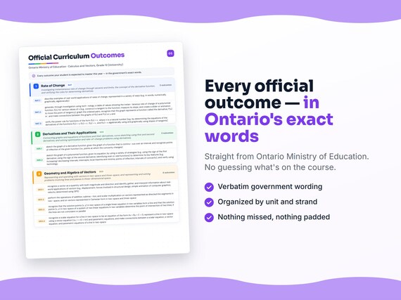
Ontario defines Calculus and Vectors, Grade 12 (University) by strands and outcomes. MapleMind teaches the same curriculum reorganized for one-skill-at-a-time tutoring — the table shows exactly where every official strand lands, and the ministry's own wording is quoted under each unit below.
Official source Ontario's official mathematics curriculumRead it on the government site — dcp.edu.gov.on.ca ↗| Official strand | Outcomes | Where MapleMind teaches it |
|---|---|---|
| Strand 1 | 21 | Rate of Change |
| Strand 2 | 11 | Derivatives and Their Applications |
| Strand 3 | 22 | Geometry and Algebra of Vectors |
Every skill below, taught one on one.
 Try the first session free
How MapleMind teaches Calculus and Vectors, Grade 12 (University) — every unit, lesson, and skill
Every skill below runs as a short session: a plain-words lesson, a worked example, solving it together, then a five-question skill check that earns up to three stars. Guided Mode keeps it teaching instead of answer-handing — turning it off needs a parent's password.
Unit 1Rate of ChangeOfficial strand · Strand 1
Investigating instantaneous rate of change through secants and limits, the concept of the derivative function, and verifying the rules for determining derivatives.
Investigating Instantaneous Rate of Change at a Point
- Real-world examples of rates of changemcv4u.1.1 — Describe examples of real-world applications of rates of change, represented in words, numerically, graphically, and algebraically.
- Connecting average rate of change to secants and instantaneous rate to tangentsmcv4u.1.2 — Describe connections between the average rate of change of a smooth function over an interval and the slope of the secant, and between the instantaneous rate of change at a point and the slope of the tangent.
- Approximating instantaneous rate of change using secants approaching the tangentmcv4u.1.3 — Make connections between an approximate instantaneous rate of change at a point and average rates of change over intervals containing the point, using secants approaching the tangent.
- Recognizing limits graphically and numericallymcv4u.1.4 — Recognize, through investigation, graphical and numerical examples of limits, and explain the reasoning involved.
- Connecting average and instantaneous rate of change to the limit expressionmcv4u.1.5 — Make connections between the average rate of change over an interval and the expression (f(a+h) − f(a))/h, and between the instantaneous rate of change at a point and the limit of that expression as h approaches zero.
- Comparing simplified and unsimplified instantaneous rate calculationsmcv4u.1.6 — Compare, through investigation, the calculation of instantaneous rates of change at a point for polynomial functions, with and without first simplifying the difference-quotient expression.
- Determining intervals where instantaneous rate of change is positive, negative, or zeromcv4u.1.7 — Determine numerically and graphically the intervals over which the instantaneous rate of change is positive, negative, or zero, and describe behaviour at and between local maxima and minima.
Investigating the Concept of the Derivative Function
- Graphing the derivative from a table of instantaneous rates of changemcv4u.1.8 — Generate, through investigation using technology, a table of values showing instantaneous rates of change of a polynomial function, graph the ordered pairs, and recognize the graph as the derivative function.
- Determining polynomial derivatives using the limit definitionmcv4u.1.9 — Determine the derivatives of polynomial functions by simplifying the algebraic expression and then taking the limit of the simplified expression as h approaches zero.
- Investigating the derivative graph of a sinusoidal functionmcv4u.1.10 — Determine, through investigation using technology, the graph of the derivative of a given sinusoidal function.
- Investigating the derivative graph of an exponential functionmcv4u.1.11 — Determine, through investigation using technology, the graph of the derivative of a given exponential function, and make connections between the graphs of the function and its derivative.
- Discovering the number e as the base where f'(x) = f(x)mcv4u.1.12 — Determine, through investigation using technology, the exponential function for which f'(x) = f(x), and identify the number e as that base.
- The natural logarithm as the inverse of the exponential function e^xmcv4u.1.13 — Recognize that the natural logarithmic function f(x) = ln x is the inverse of f(x) = e^x, and make connections between the two functions.
- Verifying the derivative of a general exponential functionmcv4u.1.14 — Verify, using technology, that the derivative of the exponential function f(x) = a^x is f'(x) = a^x ln a for various values of a.
Investigating the Properties of Derivatives
- Verifying the power rule for natural-number exponentsmcv4u.1.15 — Verify the power rule for functions of the form f(x) = x^n, where n is a natural number, both algebraically and graphically.
- Verifying the constant, constant multiple, sum, and difference rulesmcv4u.1.16 — Verify the constant, constant multiple, sum, and difference rules graphically and numerically, and read and interpret proofs of these rules.
- Determining polynomial derivatives algebraically and using them for rate-of-change problemsmcv4u.1.17 — Determine algebraically the derivatives of polynomial functions, and use these derivatives to determine the instantaneous rate of change at a point and the point(s) at which a given rate of change occurs.
- Verifying the power rule for rational exponentsmcv4u.1.18.a — Verify that the power rule applies to functions of the form f(x) = x^n where n is a rational number, by comparing slopes of tangents with values from the power rule.
- Verifying the chain rulemcv4u.1.18.b — Verify algebraically the chain rule using monomial functions, comparing the chain-rule derivative with the derivative of the simplified expanded form.
- Verifying the product rulemcv4u.1.18.c — Verify algebraically the product rule using polynomial functions, comparing the product-rule derivative with the derivative of the expanded form.
- Solving derivative problems using the product and chain rulesmcv4u.1.19 — Solve problems, using the product and chain rules, involving the derivatives of polynomial, sinusoidal, exponential, rational, radical, and other combined functions.
The official wording — 21 outcomes in this unit
- mcv4u.1.1
describe examples of real-world applications of rates of change, represented in a variety of ways (e.g., in words, numerically, graphically, algebraically)
- mcv4u.1.2
describe connections between the average rate of change of a function that is smooth (i.e., continuous with no corners) over an interval and the slope of the corresponding secant, and between the instantaneous rate of change of a smooth function at a point and the slope of the tangent at that point
- mcv4u.1.3
make connections, with or without graphing technology, between an approximate value of the instantaneous rate of change at a given point on the graph of a smooth function and average rates of change over intervals contain- ing the point (i.e., by using secants through the given point on a smooth curve to approach the tangent at that point, and determining the slopes of the approaching secants to approxi- mate the slope of the tangent)
- mcv4u.1.4
recognize, through investigation with or without technology, graphical and numerical examples of limits, and explain the reasoning involved (e.g., the value of a function approaching an asymptote, the value of the ratio of successive terms in the Fibonacci sequence)
- mcv4u.1.5
make connections, for a function that is smooth over the interval a ≤ x ≤ a + h, between the average rate of change of the function over this interval and the value of the expression , and between the instantaneous rate of change of the function at x = a and the value of the limit
- mcv4u.1.6
compare, through investigation, the calcula- tion of instantaneous rates of change at a point (a, f(a)) for polynomial functions [e.g., f(x) = x , f(x) = x ], with and without simplifying the expression before substituting values of h that approach zero
- mcv4u.1.7
determine numerically and graphically the intervals over which the instantaneous rate of change is positive, negative, or zero for a function that is smooth over these intervals (e.g., by using graphing technology to exam- ine the table of values and the slopes of tan- gents for a function whose equation is given; by examining a given graph), and describe the behaviour of the instantaneous rate of change at and between local maxima and minima
- mcv4u.1.8
generate, through investigation using tech- nology, a table of values showing the instan- taneous rate of change of a polynomial function, f(x), for various values of x (e.g., construct a tangent to the function, measure its slope, and create a slider or animation to move the point of tangency), graph the ordered pairs, recognize that the graph represents a function called the derivative, f’(x) or , and make connections between the graphs of f(x) and f’(x) or y and
- mcv4u.1.9
determine the derivatives of polynomial func- tions by simplifying the algebraic expression and then taking the limit of the simplified expression as h approaches zero
- mcv4u.1.10
determine, through investigation using tech- nology, the graph of the derivative f’(x) or of a given sinusoidal function [i.e., f(x) = sin x, f(x) = cos x] (e.g., by generating a table of values showing the instantaneous rate of change of the function for various values of x and graphing the ordered pairs; by using dynamic geometry software to verify graphi- cally that when f(x) = sin x, f’(x) = cos x, and when f(x) = cos x, f’(x) = – sin x; by using a motion sensor to compare the displacement and velocity of a pendulum)
- mcv4u.1.11
determine, through investigation using tech- nology, the graph of the derivative f’(x) or of a given exponential function [i.e., f(x) = a (a > 0, a ≠ 1)] [e.g., by generating a table of values showing the instantaneous rate of change of the function for various values of x and graphing the ordered pairs; by using dynamic geometry software to verify that when f(x) = a , f’(x) = kf(x)], and make con- nections between the graphs of f(x) and f’(x)
- mcv4u.1.12
determine, through investigation using tech- nology, the exponential function f(x) = a (a > 0, a ≠ 1) for which f’(x) = f(x) (e.g., by using graphing technology to create a slider that varies the value of a in order to deter- mine the exponential function whose graph is the same as the graph of its derivative), iden- tify the number e to be the value of a for which f’(x) = f(x)
- mcv4u.1.13
recognize that the natural logarithmic func- tion f(x) = loge x, also written as f(x) = ln x, is the inverse of the exponential function f(x) = e , and make connections between f(x) = ln x and f(x) = e
- mcv4u.1.14
verify, using technology (e.g., calculator, graphing technology), that the derivative of the exponential function f(x) = a is f’(x) = a ln a for various values of a
- mcv4u.1.15
verify the power rule for functions of the form f(x) = x , where n is a natural number [e.g., by determining the equations of the derivatives of the functions f(x) = x, f(x) = x , f(x) = x , and f(x) = x algebraically using and graphically using slopes of tangents]
- mcv4u.1.16
verify the constant, constant multiple, sum, and difference rules graphically and numeri- cally [e.g., by using the function g(x) = kf(x) and comparing the graphs of g’(x) and kf’(x); by using a table of values to verify that f’(x) + g’(x) = ( f + g)’(x), given f(x) = x and g(x) = 3x], and read and interpret proofs involving of the constant, constant multiple, sum, and difference rules
- mcv4u.1.17
determine algebraically the derivatives of polynomial functions, and use these deriva- tives to determine the instantaneous rate of change at a point and to determine point(s) at which a given rate of change occurs
- mcv4u.1.18.a
verify that the power rule applies to functions of the form f(x) = x , where n is a rational number [e.g., by comparing values of the slopes of tangents to the function f(x) = x with values of the derivative function deter- mined using the power rule]
- mcv4u.1.18.b
verify algebraically the chain rule using monomial functions [e.g., by determining the same derivative for f(x) = (5x ) by using the chain rule and by differentiating the simplified form, f(x) = 5 x]
- mcv4u.1.18.c
and the product rule using polynomial functions [e.g., by determining the same derivative for f(x) = (3x + 2)(2x – 1) by using the product rule and by differentiating the expanded form f(x) = 6x + 4x – 3x – 2]
- mcv4u.1.19
solve problems, using the product and chain rules, involving the derivatives of polynomial functions, sinusoidal functions, exponential functions, rational functions [e.g., by expressing f(x) = as the product f(x) = (x + 1)(x – 1) ], radical functions [e.g., by expressing f(x) = √x + 5 as the power f(x) = (x + 5) ], and other simple combinations of functions
Unit 2Derivatives and Their ApplicationsOfficial strand · Strand 2
Connecting graphs and equations of functions and their derivatives, curve sketching using first and second derivatives, and solving optimization and rate-of-change problems using derivatives.
Connecting Graphs and Equations of Functions and Their Derivatives
- Sketching a derivative graph and recognizing points of inflectionmcv4u.2.1 — Sketch the graph of a derivative function given the graph of a continuous function, and recognize points of inflection as points where concavity changes.
- The second derivative as the rate of change of the rate of changemcv4u.2.2 — Recognize the second derivative as the rate of change of the rate of change, and sketch the graphs of the first and second derivatives given the graph of a smooth function.
- Determining the second derivative algebraicallymcv4u.2.3.a — Determine algebraically the equation of the second derivative f''(x) of a polynomial or simple rational function f(x).
- Connecting the graphs of a function and its first and second derivativesmcv4u.2.3.b — Make connections, through investigation using technology, between the key features of the graph of a function (increasing/decreasing intervals, local maxima and minima, points of inflection, concavity) and the graphs of its first and second derivatives.
- Sketching multiple possible functions from derivative informationmcv4u.2.4 — Describe key features of a polynomial function given information about its first and/or second derivatives, sketch two or more possible consistent graphs, and explain why infinitely many graphs are possible.
Solving Problems Using Mathematical Models and Derivatives
- Sketching a polynomial graph using first/second derivative strategiesmcv4u.2.5 — Sketch the graph of a polynomial function, given its equation, by using a variety of strategies to determine its key features, and verify with technology.
- Connecting displacement, velocity, and acceleration to the derivativemcv4u.2.6 — Make connections between the concepts of displacement, velocity, and acceleration, and the concept of the derivative, in a variety of ways.
- Connecting derivatives to real-world applicationsmcv4u.2.7 — Make connections between the graphical or algebraic representations of derivatives and real-world applications such as population change, inflation, and rates of flow.
- Solving instantaneous rate-of-change problems using the derivativemcv4u.2.8 — Solve problems, using the derivative, that involve instantaneous rates of change, including problems arising from real-world applications, given the equation of a function.
- Solving optimization problemsmcv4u.2.9 — Solve optimization problems involving polynomial, simple rational, and exponential functions drawn from a variety of applications.
- Solving real-world problems using a mathematical model and the derivativemcv4u.2.10 — Solve problems arising from real-world applications by applying a mathematical model and the concepts and procedures associated with the derivative, and interpret and communicate the results.
The official wording — 11 outcomes in this unit
- mcv4u.2.1
sketch the graph of a derivative function, given the graph of a function that is continu- ous over an interval, and recognize points of inflection of the given function (i.e., points at which the concavity changes)
- mcv4u.2.2
recognize the second derivative as the rate of change of the rate of change (i.e., the rate of change of the slope of the tangent), and sketch the graphs of the first and second derivatives, given the graph of a smooth function
- mcv4u.2.3.a
determine algebraically the equation of the second derivative f”(x) of a polynomial or simple rational function f(x)
- mcv4u.2.3.b
and make connections, through investigation using technology, between the key features of the graph of the function (e.g., increasing/ decreasing intervals, local maxima and minima, points of inflection, intervals of con- cavity) and corresponding features of the graphs of its first and second derivatives (e.g., for an increasing interval of the function, the first derivative is positive; for a point of inflection of the function, the slopes of tangents change their behaviour from increasing to decreasing or from decreasing to increasing, the first derivative has a maximum or mini- mum, and the second derivative is zero)
- mcv4u.2.4
describe key features of a polynomial function, given information about its first and/or sec- ond derivatives (e.g., the graph of a deriva- tive, the sign of a derivative over specific intervals, the x-intercepts of a derivative), sketch two or more possible graphs of the function that are consistent with the given information, and explain why an infinite number of graphs is possible
- mcv4u.2.5
sketch the graph of a polynomial function, given its equation, by using a variety of strategies (e.g., using the sign of the first derivative; using the sign of the second derivative; identifying even or odd functions) to determine its key features (e.g., increasing/ decreasing intervals, intercepts, local maxima and minima, points of inflection, intervals of concavity), and verify using technology
- mcv4u.2.6
make connections between the concept of motion (i.e., displacement, velocity, accelera- tion) and the concept of the derivative in a variety of ways (e.g., verbally, numerically, graphically, algebraically)
- mcv4u.2.7
make connections between the graphical or algebraic representations of derivatives and real-world applications (e.g., population and rates of population change, prices and infla- tion rates, volume and rates of flow, height and growth rates)
- mcv4u.2.8
solve problems, using the derivative, that involve instantaneous rates of change, includ- ing problems arising from real-world applica- tions (e.g., population growth, radioactive decay, temperature changes, hours of day- light, heights of tides), given the equation of a function
- mcv4u.2.9
solve optimization problems involving poly- nomial, simple rational, and exponential func- tions drawn from a variety of applications, including those arising from real-world situations
- mcv4u.2.10
solve problems arising from real-world appli- cations by applying a mathematical model and the concepts and procedures associated with the derivative to determine mathemati- cal results, and interpret and communicate the results
Unit 3Geometry and Algebra of VectorsOfficial strand · Strand 3
Representing and operating with vectors in two-space and three-space, and representing and solving problems involving lines and planes in three-dimensional space.
Representing Vectors Geometrically and Algebraically
- A vector as a quantity with magnitude and directionmcv4u.3.1 — Recognize a vector as a quantity with both magnitude and direction, and identify, gather, and interpret information about real-world applications of vectors.
- Representing a vector in two-space geometrically and algebraicallymcv4u.3.2 — Represent a vector in two-space geometrically as a directed line segment, and algebraically, and recognize vectors with the same magnitude and direction as equal vectors.
- Converting between Cartesian form and directed line segment form for two-space vectorsmcv4u.3.3 — Determine, using trigonometric relationships, the Cartesian representation of a vector given as a directed line segment, or the directed-line-segment representation of a vector given in Cartesian form.
- Representing points and vectors in three-space and finding distance and magnitudemcv4u.3.4 — Recognize that points and vectors in three-space can be represented using Cartesian coordinates, and determine the distance between two points and the magnitude of a vector.
Operating With Vectors
- Adding, subtracting, and scalar-multiplying vectorsmcv4u.3.5 — Perform the operations of addition, subtraction, and scalar multiplication on vectors represented as directed line segments and in Cartesian form in two-space and three-space.
- Properties of vector addition, subtraction, and scalar multiplicationmcv4u.3.6 — Determine, through investigation, properties such as commutative, associative, and distributive properties of vector addition, subtraction, and scalar multiplication.
- Solving real-world problems with vector addition, subtraction, and scalar multiplicationmcv4u.3.7 — Solve problems involving the addition, subtraction, and scalar multiplication of vectors, including problems arising from real-world applications.
- The dot product and its applicationsmcv4u.3.8 — Perform the dot product on two vectors represented as directed line segments and in Cartesian form in two-space and three-space, and describe applications of the dot product.
- Properties of the dot productmcv4u.3.9 — Determine, through investigation, properties of the dot product, such as whether it is commutative, distributive, or associative.
- The cross product and its applicationsmcv4u.3.10 — Perform the cross product on two vectors in Cartesian form in three-space, determine the magnitude of the cross product, and describe its applications.
- Properties of the cross productmcv4u.3.11 — Determine, through investigation, properties of the cross product, such as whether it is commutative, distributive, or associative.
- Solving real-world problems involving the dot and cross productmcv4u.3.12 — Solve problems involving dot product and cross product, including problems arising from real-world applications.
Describing Lines and Planes Using Linear Equations
- Solution points of linear equations in two-space and their intersectionmcv4u.3.13 — Recognize that the solution points of a single linear equation in two-space form a line, and the solution points of a system of two such equations determine an intersection point.
- Solution points of linear equations in three-space as planes and their line of intersectionmcv4u.3.14 — Determine, through investigation with and without technology, that the solution points of a single linear equation in three-space form a plane, and of a system of two such equations form a line of intersection.
- Geometric configurations of up to three lines and/or planes in three-spacemcv4u.3.15 — Determine, through investigation using a variety of tools and strategies, different geometric configurations of combinations of up to three lines and/or planes, and organize them by how they intersect.
Describing Lines and Planes Using Scalar, Vector, and Parametric Equations
- Scalar, vector, and parametric equations of a line in two-spacemcv4u.3.16 — Recognize a scalar equation for a line in two-space, represent a line using a vector equation and parametric equations, and connect the three forms.
- Representing a line in three-spacemcv4u.3.17 — Recognize that a line in three-space cannot be represented by a scalar equation, and represent it using the scalar equations of two intersecting planes and using vector and parametric equations.
- The normal to a plane and geometric properties of a planemcv4u.3.18 — Recognize a normal to a plane geometrically and algebraically, and determine, through investigation, geometric properties of the plane.
- The scalar equation of a plane and finding the intersection of three planesmcv4u.3.19 — Recognize a scalar equation for a plane in three-space, determine the intersection of three planes by solving a system of three equations, and connect the algebraic and geometric configurations.
- Determining the equations of a plane from its propertiesmcv4u.3.20 — Determine, using properties of a plane, the scalar, vector, and parametric equations of a plane.
- Converting between forms of a plane's equationmcv4u.3.21 — Determine the equation of a plane in its scalar, vector, or parametric form, given another of these forms.
- Solving problems involving distances and intersections of lines and planesmcv4u.3.22 — Solve problems relating to lines and planes in three-space involving distances or intersections, and interpret the result geometrically.
The official wording — 22 outcomes in this unit
- mcv4u.3.1
recognize a vector as a quantity with both magnitude and direction, and identify, gather, and interpret information about real-world applications of vectors (e.g., displacement, forces involved in structural design, simple animation of computer graphics, velocity determined using GPS)
- mcv4u.3.2
represent a vector in two-space geometrically as a directed line segment, with directions ex- pressed in different ways (e.g., 320º; N 40º W), and algebraically (e.g., using Cartesian coordi- nates; using polar coordinates), and recognize vectors with the same magnitude and direc- tion but different positions as equal vectors
- mcv4u.3.3
determine, using trigonometric relationships [e.g., x = rcosθ, y = rsinθ, θ = tan ( )or tan ( )+180º, r = √x + y ], the Cartesian representation of a vector in two-space given as a directed line segment, or the representation as a directed line segment of a vector in two-space given in Cartesian form [e.g., representing the vector (8, 6) as a directed line segment]
- mcv4u.3.4
recognize that points and vectors in three-space can both be represented using Cartesian coor- dinates, and determine the distance between two points and the magnitude of a vector using their Cartesian representations
- mcv4u.3.5
perform the operations of addition, subtrac- tion, and scalar multiplication on vectors represented as directed line segments in two- space, and on vectors represented in Cartesian form in two-space and three-space
- mcv4u.3.6
determine, through investigation with and without technology, some properties (e.g., commutative, associative, and distributive properties) of the operations of addition, subtraction, and scalar multiplication of vectors
- mcv4u.3.7
solve problems involving the addition, sub- traction, and scalar multiplication of vectors, including problems arising from real-world applications
- mcv4u.3.8
perform the operation of dot product on two vectors represented as directed line segments (i.e., using a•b =|a| |b|cosθ) and in Cartesian form (i.e., using a•b = a 1 b 1 + a 2 b 2 or a•b = a 1 b 1 + a 2 b 2 + a 3 b 3 ) in two-space and three-space, and describe applications of the dot product (e.g., determining the angle between two vectors; determining the projec- tion of one vector onto another)
- mcv4u.3.9
determine, through investigation, properties of the dot product (e.g., investigate whether it is commutative, distributive, or associative; investigate the dot product of a vector with itself and the dot product of orthogonal vectors)
- mcv4u.3.10
perform the operation of cross product on two vectors represented in Cartesian form in three-space [i.e., using a x b = (a 2 b 3 – a 3 b 2 , a 3 b 1 – a 1 b 3 , a 1 b 2 – a 2 b 1 )], determine the magnitude of the cross product (i.e., using|a x b|=|a| |b|sinθ), and describe applications of the cross product (e.g., deter- mining a vector orthogonal to two given vec- tors; determining the turning effect [or torque] when a force is applied to a wrench at differ- ent angles)
- mcv4u.3.11
determine, through investigation, properties of the cross product (e.g., investigate whether it is commutative, distributive, or associative; investigate the cross product of collinear vectors)
- mcv4u.3.12
solve problems involving dot product and cross product (e.g., determining projections, the area of a parallelogram, the volume of a parallelepiped), including problems arising from real-world applications (e.g., determin- ing work, torque, ground speed, velocity, force)
- mcv4u.3.13
recognize that the solution points (x, y) in two-space of a single linear equation in two variables form a line and that the solution points (x, y) in two-space of a system of two linear equations in two variables determine the point of intersection of two lines, if the lines are not coincident or parallel
- mcv4u.3.14
determine, through investigation with technol- ogy (i.e., 3-D graphing software) and without technology, that the solution points (x, y, z) in three-space of a single linear equation in three variables form a plane and that the solution points (x, y, z) in three-space of a system of two linear equations in three variables form the line of intersection of two planes, if the planes are not coincident or parallel
- mcv4u.3.15
determine, through investigation using a variety of tools and strategies (e.g., modelling with cardboard sheets and drinking straws; sketching on isometric graph paper), different geometric configurations of combinations of up to three lines and/or planes in three-space (e.g., two skew lines, three parallel planes, two intersecting planes, an intersecting line and plane); organize the configurations based on whether they intersect and, if so, how they intersect (i.e., in a point, in a line, in a plane)
- mcv4u.3.16
recognize a scalar equation for a line in two-space to be an equation of the form Ax + By + C = 0, represent a line in two-space using a vector equation (i.e., r = r0 + tm) and parametric equations, and make connections between a scalar equation, a vector equation, and parametric equations of a line in two-space
- mcv4u.3.17
recognize that a line in three-space cannot be represented by a scalar equation, and rep- resent a line in three-space using the scalar equations of two intersecting planes and using vector and parametric equations (e.g., given a direction vector and a point on the line, or given two points on the line)
- mcv4u.3.18
recognize a normal to a plane geometrically (i.e., as a vector perpendicular to the plane) and algebraically [e.g., one normal to the plane 3x + 5y – 2z = 6 is (3, 5, –2)], and deter- mine, through investigation, some geometric properties of the plane (e.g., the direction of any normal to a plane is constant; all scalar multiples of a normal to a plane are also nor- mals to that plane; three non-collinear points determine a plane; the resultant, or sum, of any two vectors in a plane also lies in the plane)
- mcv4u.3.19
recognize a scalar equation for a plane in three-space to be an equation of the form Ax + By + Cz + D = 0 whose solution points make up the plane, determine the intersection of three planes represented using scalar equations by solving a system of three linear equations in three unknowns algebraically (e.g., by using elimination or substitution), and make connections between the algebraic solution and the geometric configuration of the three planes
- mcv4u.3.20
determine, using properties of a plane, the scalar, vector, and parametric equations of a plane
- mcv4u.3.21
determine the equation of a plane in its scalar, vector, or parametric form, given another of these forms
- mcv4u.3.22
solve problems relating to lines and planes in three-space that are represented in a variety of ways (e.g., scalar, vector, parametric equa- tions) and involving distances (e.g., between a point and a plane; between two skew lines) or intersections (e.g., of two lines, of a line and a plane), and interpret the result geometrically
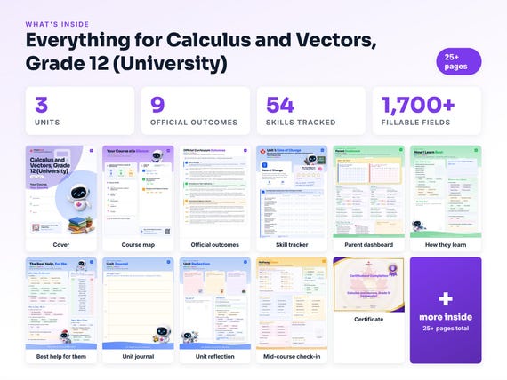

Printable workbook · A keepsake of the year
A Calculus and Vectors, Grade 12 (University) workbook worth keeping
Built from the same official curriculum as this page. Before and after each skill above, your student colours in how sure they feel — so the two of you can see, on one page, what's clicking and what needs another look. It's a quiet way to follow how the year is really going.
By June it's full of their own handwriting: units worked through, confidence grown, a mid-year check-in, notes from parent-teacher night, and a certificate at the end. Less a worksheet, more a record of the year worth keeping on the shelf.
Instant download · see every page, reviews and the full description · five or more workbooks are $2.99 each
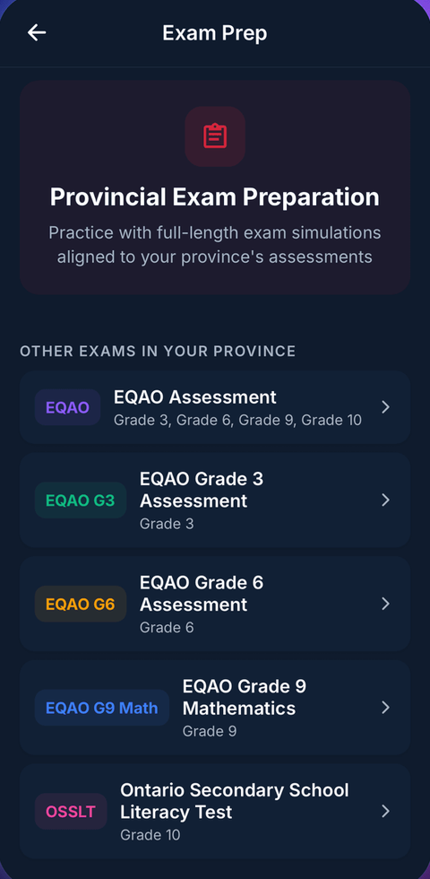
What it looks like in the app


Common questions
Can MapleMind help me with Calculus and Vectors, Grade 12 (University)?
Yes. MapleMind's AI tutor covers all 54 skills in Ontario's Calculus and Vectors, Grade 12 (University) — you pick the exact skill, and the tutor teaches it step by step: a short lesson, a worked example, solving together, then a skill check to show it stuck.
Is MapleMind aligned to Ontario's official curriculum?
Yes. Every skill in this course maps to an official outcome code from Ontario's Grade 12 Mathematics curriculum, and the ministry's own wording is quoted under each unit on this page — with the official government source linked so you can check it yourself.
What does MapleMind cost?
It's free to start — 5 tutoring chats and a practice quiz every day, no credit card. A Pro subscription ($9.99/month or $49.99/year CAD, 7-day free trial) unlocks unlimited tutoring, practice, and exam simulations.
What if I'm stuck on just one topic?
That's the point of skill-level tutoring: open Calculus and Vectors, Grade 12 (University) in the app, tap the exact skill from the list on this page, and the tutor teaches just that — no wading through lessons you don't need.
Does MapleMind work in French or other languages?
Yes — 14 languages, including French. Both the app and the tutor's explanations switch to the language you choose.
Where can I see the official Ontario curriculum for Calculus and Vectors, Grade 12 (University)?
The official source is linked on this page — Ontario's official mathematics curriculum. The outline here follows it: every MapleMind skill carries its official outcome code, and the ministry's own wording is quoted under each unit.
Keep exploring
Ready when you are
Pick a skill from this page and see it taught properly — free, in the browser, in under a minute.